Switch from VLOOKUP to XLOOKUP in minutes. Learn exact vs approximate matches, left‑lookups, wildcards, multi‑criteria, and 2D lookups—with copy‑paste formulas and a sample workbook.
TL;DR
Products).- XLOOKUP replaces VLOOKUP and HLOOKUP with one function that’s direction‑agnostic, easier to read, and more robust (no “column number” to break).
- Use XLOOKUP for exact, approximate, left‑lookups, wildcards, multi‑criteria, and 2D lookups.
- Grab the sample workbook and formulas below to practice right away.
Download: XLOOKUP vs VLOOKUP – Sample Workbook →
xlookup-vs-vlookup-sample.xlsx
When to switch (and why people get burned by VLOOKUP)
- VLOOKUP needs a column number. If someone inserts a column, your result shifts and breaks silently.
- VLOOKUP only looks right. If your key is not the leftmost column, you’re stuck or need a helper column.
- XLOOKUP fixes both: you point to key column and return column(s) directly. It also supports not‑found messages, approximate matches, and wildcards—all in one place.
Sample data you’ll use
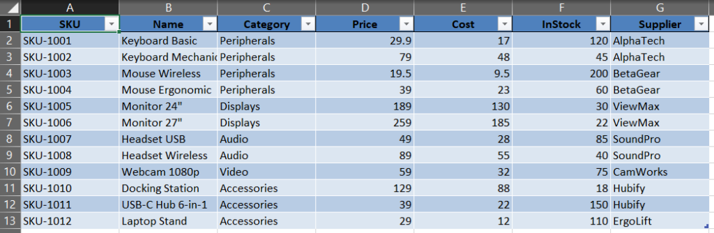
In the workbook, Products is a proper Excel Table with columns:
SKU | Name | Category | Price | Cost | InStock | SupplierYou’ll practice on the Examples sheet. (If you don’t want to download, just recreate a small table with 10–12 rows.)
The 6 patterns you’ll reuse
1) Exact match (the default)
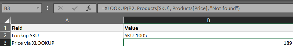
Goal: Find the price for a given SKU.
=XLOOKUP(B2, Products[SKU], Products[Price], "Not found")B2= lookup SKU (e.g.,SKU-1005)- If the SKU doesn’t exist, you’ll see Not found (no extra IFERROR needed).
VLOOKUP equivalent (fragile):
=IFERROR(VLOOKUP(B2, Products[#All], 4, FALSE), "Not found")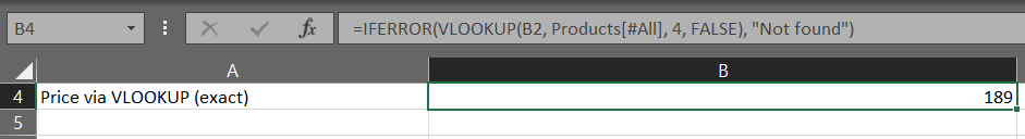
Breaks if columns move, because
4means “fourth column”.
2) Left lookup (VLOOKUP can’t)
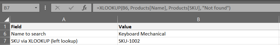
Goal: Given a Name, return the SKU (which sits left of Name).
=XLOOKUP(B6, Products[Name], Products[SKU], "Not found")XLOOKUP can return from any direction because you choose the return array explicitly.
3) Wildcards (contains/starts/ends with)
Goal: First match for names containing “Headset”.
=XLOOKUP("*Headset*", Products[Name], Products[SKU], "Not found", 2)2= wildcard match.- Use
*text*(contains),text*(starts with),*text(ends with).
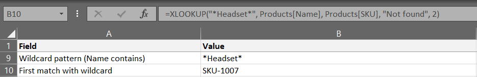
*Headset* returns the first match.4) Approximate match (price tiers, bands)
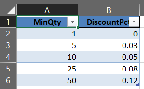
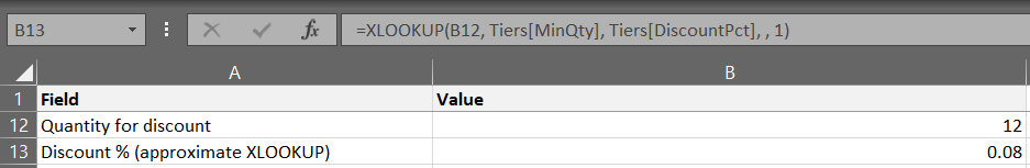
Goal: Return a discount based on Quantity, using the largest MinQty that’s ≤ Quantity.
=XLOOKUP(B12, Tiers[MinQty], Tiers[DiscountPct], , 1)1= next smaller (approximate) match.- Your
Tiers[MinQty]column should be sorted ascending.
5) Multi‑criteria lookup (no helper column needed)
Goal: Find Price where Name AND Category both match.
=XLOOKUP(B15, Products[Name] & "|" & Products[Category], Products[Price], "Not found")- Build a key
Name|Categoryin the formula and in the lookup cell (e.g.,Mouse Wireless|Peripherals). - For more criteria, extend the concatenation the same way.
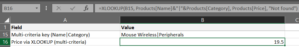
Name|Category to match two fields at once.6) 2D lookup (choose the column to return at runtime)
Goal: User picks a Field (e.g., Price/Cost/Supplier), return that field for the chosen SKU.
=LET(
  headers, Products[#Headers],
  data,    Products[#Data],
  sku,     B14,
  field,   B15,
  rowvals, XLOOKUP(sku, Products[SKU], data),
  col,     XMATCH(field, INDEX(headers,1,0)),
  INDEX(rowvals, col)
)LETnames the pieces so the formula is readable.XMATCHfinds which column index the chosen field represents.

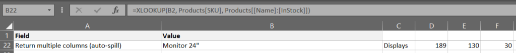
“Return multiple columns” in one go (spilling)
Want Name, Price, InStock side‑by‑side? Select the top‑left target cell and use:
=XLOOKUP(B2, Products[SKU], Products[[Name]:[InStock]])If your Excel supports dynamic arrays (Microsoft 365/2021+), the results will spill across the next columns automatically.
Common errors & quick fixes
- #N/A / Not found: Check spaces, exact spelling, or use wildcards if it’s a contains search.
- Wrong result after inserting a column (VLOOKUP): switch to XLOOKUP (or
INDEX/MATCH) to avoid column‑number fragility. - Approximate match returns unexpected tier: confirm your MinQty is sorted ascending and your
match_modeis 1 (next smaller). - Slow with very large tables: turn your range into an Excel Table, avoid full‑column references, and filter the source where you can.
- Dynamic arrays not spilling: you may be on an older Excel—test with
=SEQUENCE(3); if it doesn’t spill, upgrade to Microsoft 365/2021.
Copy‑paste cheat sheet
-- Exact price by SKU
=XLOOKUP(SKU, Products[SKU], Products[Price], "Not found")

-- Left lookup (Name -> SKU)
=XLOOKUP(NameCell, Products[Name], Products[SKU], "Not found")

-- Wildcard contains
=XLOOKUP("*keyword*", Products[Name], Products[SKU], "Not found", 2)

-- Approximate (quantity tiers, next smaller)
=XLOOKUP(Qty, Tiers[MinQty], Tiers[DiscountPct], , 1)

-- Multi-criteria (Name + Category)
=XLOOKUP(Name&"|"&Category, Products[Name]&"|"&Products[Category], Products[Price], "Not found")

-- 2D lookup (choose the field)
=LET(h,Products[#Headers], d,Products[#Data], r,XLOOKUP(SKU,Products[SKU],d), c,XMATCH(Field,INDEX(h,1,0)), INDEX(r,c))

-- Spill multiple columns (Name..InStock)
=XLOOKUP(SKU, Products[SKU], Products[[Name]:[InStock]])
Download
- Sample workbook (.xlsx): xlookup-vs-vlookup-sample.xlsx
Open the Examples sheet and change the input cells (yellow rows) to see each pattern in action.
FAQ
Not really. XLOOKUP is simpler and more robust.
No. It’s in Microsoft 365 and Excel 2021+.
Use XLOOKUP; point return_array to any column.
Leave a Reply